Previous chapter: A Remark on Undetermined Games
This is a learning note of a course in CISPA, UdS. Taught by Bernd Finkbeiner
Introduction
Infinite games allow us to reason elegantly about infinite trees. A famous example of an argument that became significantly simpler with the introduction of game-theoretic ideas is the proof of Rabin’s theorem.
Rabin’s theorem states that the satisfiability of monadic second-order logic with two successors (S2S) is decidable. Like in Section 6, where we showed that S1S formulas can be translated to automata, we will show that S2S formulas can be translated to automata, this time, in order to accommodate more than one successor function, to automata over infinite trees.
The most difficult part of the proof of Rabin’s theorem is to show that tree automata are closed under complement. The original proof was purely combinatorial (and very difficult to understand), but the game-theoretic argument is simply based on the determinacy of the acceptance game of the tree automaton:
the acceptance of a tree by a tree automaton = the existence of a winning strategy for Player 0,
the non-acceptance = the absence of such a strategy = the existence of a winning strategy for Player 1.
We can therefore complement the language of a given tree automaton by constructing a new automaton that verifies the existence of a winning strategy for Player 1. We begin this section with a discussion of tree automata. The logic S2S and the translation to tree automata will be introduced later in the section.
Tree Automata
We consider tree automata over infinite binary trees. We use the notation for trees introduced in Section 7.1. The (full) binary tree is the language $\mathcal{T} =\lbrace 0, 1\rbrace^\ast$. For an alphabet $\Sigma, \mathcal{T}_\Sigma = \lbrace(\mathcal{T}, t)\mid t:\mathcal{T}\rightarrow\Sigma\rbrace$ is the set of all binary $\Sigma$-labeled trees.
$\textbf{Definition 12.1. } \text{An }\textit{automaton over infinite binary trees }\mathcal{A}\text{ is a tuple }(\Sigma,Q,q_0,T,Acc)\text{, where}\newline
\begin{array}{l}
\hspace{1cm} \cdot \ \Sigma \text{ is a finite alphabet,} \newline
\hspace{1cm} \cdot \ Q \text{ is a finite set of states,} \newline
\hspace{1cm} \cdot \ q_0 \in Q \text{ is an initial states,} \newline
\hspace{1cm} \cdot \ T \subseteq Q \times \Sigma \times Q \times Q, \newline
\hspace{1cm} \cdot \ Acc \subseteq Q^\omega \text{ is the accepting condition}
\end{array}$
In the following, we will refer to automata over infinite binary trees simply as tree automata. Note that a transition of a tree automaton has two successor states, rather than a successor state as for word automata. The two states correspond to the two directions 0 and 1 of the input tree, the automaton may transition into different states for the different directions.
$\textbf{Definition 12.2. } \text{A }\textit{run }\text{of a tree automata }\mathcal{A}\text{ on an infinite }\Sigma\text{-labeled binary tree }(\mathcal{T},t)\newline\text{ is a }Q\text{-labeled binary tree }(\mathcal{T},r)\text{ such that the following hold:}\newline
\begin{array}{l}
\hspace{0.5cm} \cdot \ r(\varepsilon)=q_0 \hspace{2.5cm} \cdot \ (r(n),t(n),r(n0),r(n1))\in T\text{ for all }n\in\lbrace 0,1\rbrace^\ast
\end{array}$
Note that $n0$ and $n1$ are the children of node $n$ in direction 0 and 1, respectively. The accepting runs are defined as for alternating automata in Section 7.1: we apply the acceptance condition to the branches of the run tree. (Note that a run of an alternating automaton may have finite and infinite branches. The acceptance condition is only checked on infinite branches. Here, all branches are infinite.)
$\textbf{Definition 12.3. } \text{A }\textit{run }(\mathcal{T},r)\text{ is }\textit{accepting}\text{ iff, for every infinite branch }n_0n_1n_2\dots,$
$$r(n_0)r(n_1)r(n_2)\dots\in Acc$$
The language of the tree automaton $\mathcal{A}$ consists of the set of accepted $\Sigma$-labeled trees.
Example
The following Büchi tree automaton $\mathcal{A}=(\Sigma,Q,q_0,T,\small\text{BÜCHI}\normalsize(F))$ accepts all $\lbrace a,b\rbrace$-labeled trees with infinitely many $b$’s on each branch.
- $\Sigma = \lbrace a,b\rbrace$
- $Q=\lbrace q_a,q_b\rbrace; q_0=q_a$
- $T=\lbrace(q_a,a,q_a,q_a),(q_b,a,q_a,q_a),(q_a,b,q_b,q_b),(q_b,b,q_b,q_b)\rbrace$
- $F = \lbrace q_b\rbrace$
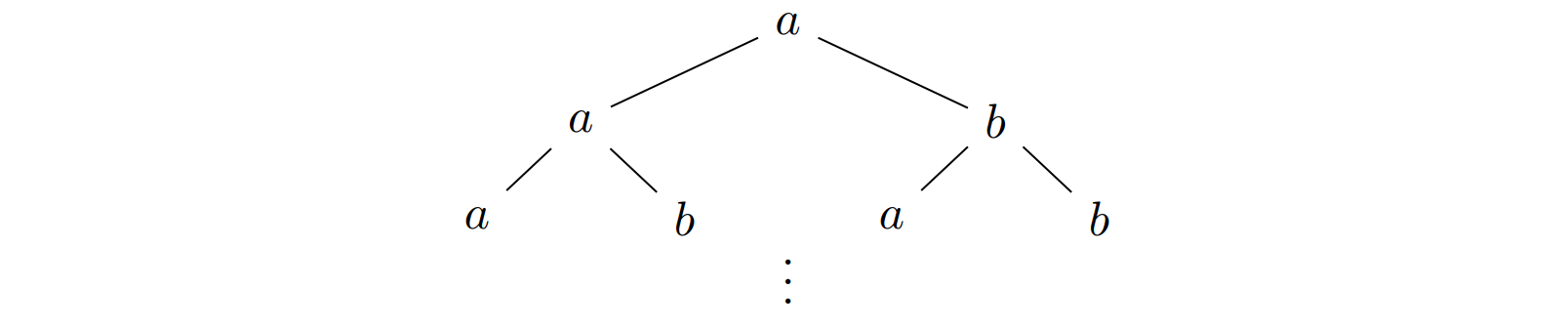
Consider the $\Sigma$-labeled input tree $(\mathcal{T},t)$:
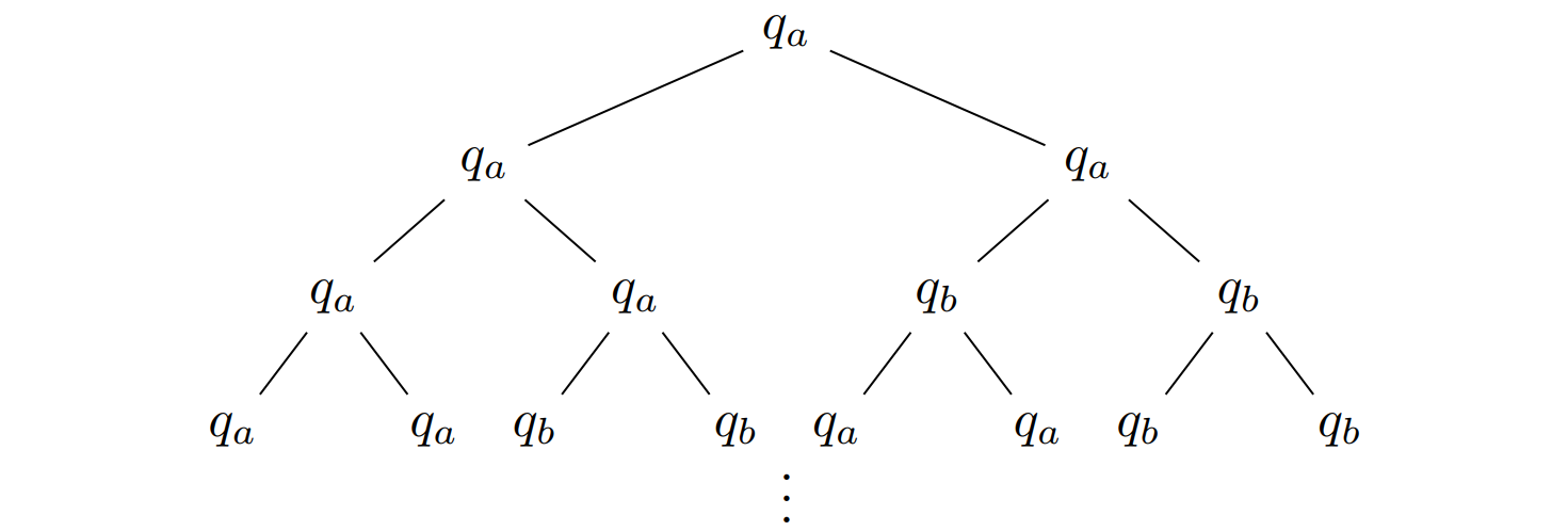
The following $Q$-labeled tree is a run $(\mathcal{T},r)$ of $\mathcal{A}$ on $(\mathcal{T},t)$:
Acceptance Game
The acceptance mechanism of a tree automaton is also characterized via its acceptance game. Player 0 can choose the alphabet $t(w)$ and Player 1 can choose the next state $q’$:
$\textbf{Definition 12.4. } \text{Let }\mathcal{A}=(\Sigma,Q,q_0,T,Acc)\text{ be a tree automata and let }(\mathcal{T},t)\text{ be a }\Sigma\text{-labeled}\newline\text{binary tree. Then the }\textit{acceptance game}\text{ of }\mathcal{A}\text{ on }(\mathcal{T},t)\text{ is the game }\mathcal{G}_{\mathcal{A},t}=(\mathcal{A}’,\text{Win}’)\text{ with the}\newline\text{infinite game arena }\mathcal{A}’=(V’,V_0’,V_1’,E’)\text{ and the winning condition Win’ defined as follows:}\newline
\begin{array}{lll}
\hspace{1cm} \cdot \ V_0’&=&\lbrace(w,q)\mid w\in\lbrace0,1\rbrace^\ast,q\in Q\rbrace\newline
\hspace{1cm} \cdot \ V_1’&=&\lbrace(w,\tau)\mid w\in\lbrace0,1\rbrace^\ast,\tau\in T\rbrace\newline
\hspace{1cm} \cdot \ E’&=&\lbrace((w,q),(w,\tau))\mid\tau=(q,t(w),q^0,q^1),\tau\in T\rbrace\ \cup \newline
&&\lbrace((w,\tau),(w,q’))\mid\tau=(q,\sigma,q^0,q^1)\text{ and}\newline
&&\hspace{3.65cm}w’=w0\text{ and }q’=q^0\text{ or }w’=w1\text{ and }q’=q^1\rbrace\newline
\hspace{1cm} \cdot \ \text{Win}’ &=& \lbrace(w[0,0],q(0))(w[0,0],\tau(0))(w[0,1],q(1))(w[0,1],\tau(1))\dots\mid\newline
&& \hspace{1cm} q(0)q(1)\dots\in Acc, w(0)w(1)\dots\in\lbrace 0,1\rbrace^\omega,\tau(0)\tau(1)\dots\in T^\omega\rbrace
\end{array}$
Example
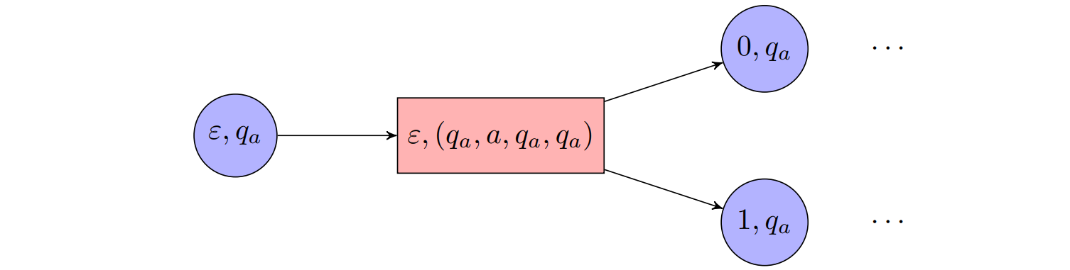
The following is a part of the acceptance game of automaton $\mathcal{A}$ from the example above:
$\textbf{Theorem 12.1. } \textit{A tree automaton }\mathcal{A}=(\Sigma,Q,q_0,T,Acc)\textit{ accepts an input tree }(\mathcal{T},r)\newline\textit{ if and only if Player 0 wins the acceptance game }\mathcal{G}_{\mathcal{A},t}=(\mathcal{A}’,\text{Win}’)\textit{ from position }(\varepsilon,q_0).$
Proof
If the input tree is accepted, there is a winning strategy for Player 0
Given an accepting run $(\mathcal{T},r)$ of $\mathcal{A}$, we construct a memoryless winning strategy $\sigma:V_0’\rightarrow V’$ for Player 0:
$$\sigma(w,q)=(w,(r(w),t(w),r(w0),r(w1)))$$
If there is a winning strategy for Player 0, the input tree is accepted
Given a winning strategy $\sigma:V’^\ast V_0’\rightarrow V’$, we construct an accepting run $(\mathcal{T},r)$ where $r(\varepsilon)=q_0$ and for all $w\in\lbrace 0,1 \rbrace^\ast$
$$r(w0)=q\text{ for }\sigma(\Delta(w))=(w,(\rule{0.5em}{0.4pt},\rule{0.5em}{0.4pt},q,\rule{0.5em}{0.4pt}))\ \text{ and }\ r(w1)=q\text{ for }\sigma(\Delta(w))=(w,(\rule{0.5em}{0.4pt},\rule{0.5em}{0.4pt},\rule{0.5em}{0.4pt}q))$$
where $\Delta(\varepsilon)=(\varepsilon,q_0)\ \text{ and }\ \Delta(wd)=\Delta(w)\cdot\sigma(\Delta(w))\cdot(wd,r(wd))\text{ for }d\in\lbrace0,1\rbrace.$
Next chapter: Emptiness Game
Please cite the source for reprints, feel free to verify the sources cited in the article, and point out any errors or lack of clarity of expression. You can comment in the comments section below or email to GreenMeeple@yahoo.com