Previous chapter: Automata-based LTL Model Checking with Sequential Circuits

This is a learning note of a course in CISPA, UdS. Taught by Bernd Finkbeiner

Introduction

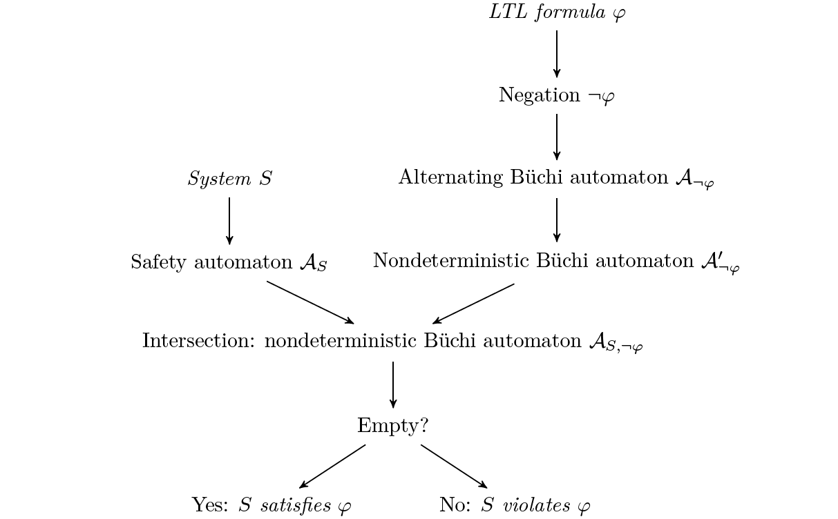
We now develop an algorithm for checking whether the language of a given Büchi automaton is empty. A natural idea is to use depth-first search (DFS) twice.

The language is non-empty $\Leftrightarrow$ it is accepted by some words:

1. there exists an accepting state $q$,
2. $q$ is reachable from some initial state (discovered by 1st DFS), and
3. $q$ can again be reached from $q$ (discovered by 2nd DFS),

Example (Simple DFS)

Consider the following Büchi automaton (edge labels do not matter and are omitted).

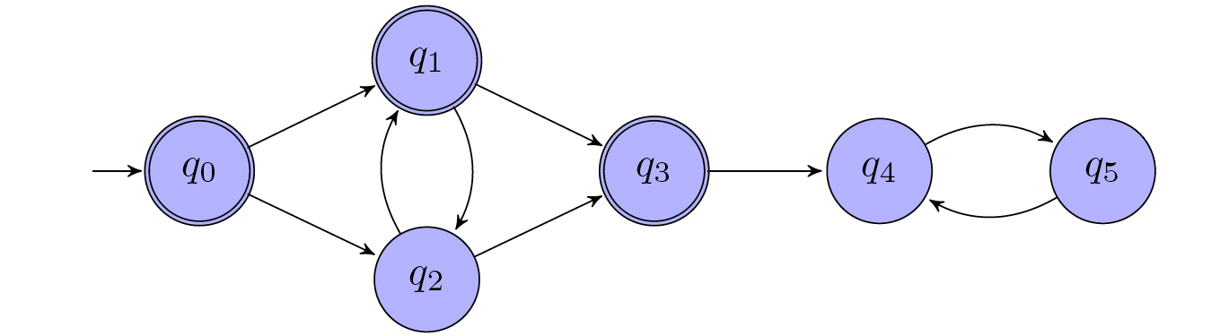
Step 1: discovers $q_0$, $q_1$, and $q_3$.
Step 2: searches from $q_0$ and $q_3$: not successful; searches from $q_1$: discovers the path back to $q_1$ via $q_2$.

Previous chapter: From Linear Arithmetic to Automata

This is a learning note of a course in CISPA, UdS. Taught by Bernd Finkbeiner

Right hand side: Hondeterministic Büchi automata

In order to find system executions that violate a given LTL formula (1), we negate the formula (2) and build an automaton that is equivent to the negated formula. For this, we can use the translaton from LTL to alternating automata (3) from Construction 7.1 followed by the Miyano-Hayashi translation from alternating Büchi automata to nondeterministic Büchi automata (4) from Construction 7.2.

Left hand side: Safety Automaton

We represent the system (1) executions as a Safety Automaton (2), which is then intersected (using Construction 3.2 with the Büchi automaton for the negated LTL formula. The actual search for a violating execution then happens as the emptiness check of the resulting Büchi automaton. In the remainder of this section, we first quickly discuss the representation of the system as a Safety Automaton, using sequential circuits as an example, and then focus on the emptiness check of Büchi automata.

Model Checking Sequential Circuits

As an illustration of how automata can be used to represent system behaviors, we consider the representation of sequential circuits to safety automata. For a more general discussion of how to represent different types of systems, such as protocols or software, we refer the reader to textbooks on model checking, such as Principles of Model Checking by Baier and Katoen.

Sequential Circuits

Previous chapter: Homogenous Inequality Testing is Automatic

This is a learning note of a course in CISPA, UdS. Taught by Bernd Finkbeiner

Introduction

With all the setup in the previous sections, We are now ready to prove the main result of this chapter.

$\textbf{Theorem 8.1. }\textit{Let }\varphi\textit{ be a linear arithmetic formula. We can effectively construct a Büchi}$ $\textit{Automaton }\mathcal{A}\textit{ such that }\mathcal{L(A)}=\lbrace\alpha_\sigma\mid\sigma\models\varphi\rbrace$

We follow the same strategy as for the analogous result for S1S in Section 6.7.

1. Introduce a logic with a (slightly) restricted syntax from S1S,
2. Show that the restriction does not come at the cost of expressive power, and
3. Use structural induction on restricted-syntax formulas to construct our desired automata.

Restricted Linear Arithmetic

The formulas of syntactically restricted linear arithmetic are defined by the following grammar:

$$\varphi::=z=1\mid g_1x_1+\dots+g_\ell x_\ell\leq h_1 y_1+\dots+h_m y_m\mid\neg\varphi\mid\varphi\wedge\varphi\mid\exists x.\varphi$$

Previous chapter: Translation from Linear Arithmetic to Automata

This is a learning note of a course in CISPA, UdS. Taught by Bernd Finkbeiner

Introduction

In the previous section, we used $x+y=z$ as an example. By extend that into a more general inequality

$$g_1x_1+\dots+g_\ell x_\ell\leq h_1y_1+\dots +h_my_m$$

where $x_1,\dots,x_\ell,y_1,\dots,y_m$ are free variables, and $g_1,\dots,g_\ell,h_1,\dots,h_m$ are positive integer constants. Such inequality can be described by a Büchi automaton.

$\textbf{Lemma 8.1. }\textit{Let }\lbrace x_1,\dots,x_\ell,y_1,\dots,y_m\rbrace\textit{ be a set of free variables, and let }g_1,\dots,g_\ell,h_1,\dots,h_m$ $\textit{be positive integer constants. There exists a Büchi automaton }\mathcal{A}\textit{ such that}$

$$\mathcal{L(A)}=\lbrace\alpha_\sigma\mid\sigma\models g_1x_1+\dots+g_\ell g_\ell\leq h_1 y_1+\dots+h_m y_m\rbrace$$

It is easy to start with constructing an automaton $\mathcal{A}_{\textsf{valid},\ell+m}$ that checks whether the word $\alpha_\sigma$ is well-formed:

1. checks that the separation symbol $({$},\dots,{$})$ occurs exactly once, and
2. the separation symbol does not appear at the beginning of the word.

A Generalize Example

Previous chapter: Encoding real numbers

This is a learning note of a course in CISPA, UdS. Taught by Bernd Finkbeiner

In this section, we will illustrate the key ideas in the translation from linear arithmetic to automata through a simple example.

Consider the formula $x+y=z$ and the following encoding of the valuation $x\mapsto1$, $y\mapsto1$, $z\mapsto2$:

$$\alpha_\sigma=\begin{bmatrix}0\newline 0\newline 0\end{bmatrix}\begin{bmatrix}0\newline 0\newline 1\end{bmatrix}
\begin{bmatrix}0\newline 0\newline 0\end{bmatrix}\begin{bmatrix}{$}\newline {$}\newline {$}\end{bmatrix}\left(\begin{bmatrix}1\newline 1\newline 0\end{bmatrix}\right)^\omega = \begin{bmatrix}x\newline y\newline z\end{bmatrix} = \begin{bmatrix}1\newline 1\newline 2\end{bmatrix}$$

Homogeneity

A equation is homogenous if there are no constant terms. The key property of homogeneity is that we can simply scaling without being unbounded. In other words, for a homogenous equation $D$, we have:

$D∼0$ (where $∼$ is an arbitrary (in)equality) if and only if, for all $k\in\mathbb{Z},2^k\cdot D∼0$. (Scaling behaviour)

As we can see the equation $x+y=z$ is homogenous, i.e., $D: x+y−z = 0$ and $2^k\cdot x+2^k\cdot y−2^k\cdot z∼0$

We immediately observe that:

Previous chapter: Linear Arithmetic (Theory)

This is a learning note of a course in CISPA, UdS. Taught by Bernd Finkbeiner

Introduction

In last section, we have seen the definiton of Linera Arithmetic, which is similar to S1S. Let see how we can apply it in math and moreover, the connection between logic and automata.

Encoding Real Numbers

We can encode any real number $x\in\mathbb{R}$ into the form $(0+1)(0+1)^\ast{$}(0+1)^\omega$ in two steps:

Step 1

For a real number $x\in\mathbb{R}$, represent it as a pair $(x_I,x_F)$ so that $x=x_I+x_F$.
integer part = $x_I\in\mathbb{Z}$, and fractional part = $x_F\in[0, 1]$, a real number between $0$ and $1$ (both inclusive)

For example, the $1.5 = (1, 0.5)$, and $-{2\over 3}=(−1, {1\over3})$. Note that integers always have two different representations depends on setting the fractional part as $0$ or $1$, and Negative sign can only be represented using the integer part. For example $3=(2,1)$ or $(3,0)$

Step 2

Previous chapter: Translating Alternating to Nondeterministic automata

This is a learning note of a course in CISPA, UdS. Taught by Bernd Finkbeiner

Introduction

In the previous sections, we have seen that the automata machinery can be applied to logical problems by translating formulas into automata. We now study another application of the powerful connection between logic and automata, this time in the setting of real numbers.

Theory of Linear Arithmetic

Definitions and Semantics

Let $V$ be a set of (first-order) variables. The terms of linear arithmetic are defined by the following grammar:

$$t::=0\mid1\mid x\mid t+t$$

The formulas of linear arithmetic are defined by the following grammar, where $x\in V$ is a variable:

$$\varphi::=t\leq t\mid\neg\varphi\mid\varphi\wedge\varphi\mid\exists x.\varphi$$

Previous chapter: From LTL to Alternating Büchi Automata

This is a learning note of a course in CISPA, UdS. Taught by Bernd Finkbeiner

Introduction

The translation from alternating to nondeterministic automata is based on a representation of runs as directed acyclic graphs (DAGs). The idea is similar to the DAG representation we used in the complementation construction for nondeterministic Büchi automata in Section 5.

There the DAG was used to represent the set of all runs of the nondeterministic automaton. The complement automaton would then ”guess” the DAG level-by-level. Here, the DAG is used to represent the branches of a (single) run of the alternating automaton. The idea is illustrated in the following example.

Example

$\textbf{Definition 7.5. } \text{ A } \textit{run DAG }\text{ of an alternating Büchi automaton }\mathcal{A}\text{ on an infinite word }\alpha\text{ is a}$ $\text{DAG }(V,E)\text{, with }V\subseteq Q\times\mathbb{N}\text{ and }(q_0,0)\in V\text{, where}$

$\begin{array}{ll} \hspace{0.5cm} \cdot & E\subseteq \bigcup_{i\in\mathbb{N}}(Q\times\lbrace i\rbrace)\times(Q\times\lbrace i+1\rbrace) \newline \hspace{0.5cm} \cdot & \forall(q,i)\in V \ . \ \exists Y\subseteq Q\text{ s.t. } \newline & Y\models\delta(q,\alpha(i)),Y\times\lbrace i+1\rbrace\subseteq V\text{ and }\lbrace(q,i)\rbrace\times (Y\times\lbrace i+1\rbrace)\subseteq E.\end{array}$

• Every vertices are expressed in (state, letter index)
• Edges are all possible paths from current state $q$

A run DAG is accepting if every infinite path has infinitely many visits to $F\times\mathbb{N}$.

Previous chapter: Alternating Büchi Automata

This is a learning note of a course in CISPA, UdS. Taught by Bernd Finkbeiner

Introduction

It is usually much simpler to translate a logical formula into an alternating automaton than into a nondeterministic automaton. We illustrate this with the translation of LTL formulas into equivalent alternating Büchi automata. The states are simply the subformulas of the given formula and their negations (this set is called the closure of the formula). The transition function is derived from the expansion laws of the logic.

For example, an Until formula $\varphi_1\ \mathcal{U}\ \varphi_2$ holds if:

• $\varphi_2$ holds or
• $\varphi_1$ holds and the entire formula holds in the next step.

The boolean formula produced by the transition function from the state $\varphi_1\ \mathcal{U}\ \varphi_2$ is therefore:

• a disjunction $(\wedge)$ between the transition function for $\varphi_2$ and
• a conjunction $(\vee)$ between the transition function for $\varphi_1$ and the state $\varphi_1\ \mathcal{U}\ \varphi_2$.

From LTL to Alternating Automata

$\textbf{Construction 7.1. }\text{Let }\varphi\text{ be an LTL formula. We construct the alternating Büchi automaton }$ $\mathcal{A_\varphi}=(\Sigma,Q,\varphi,\delta,\small\text{BÜCHI} \normalsize(F))\text{ using:}$

$\begin{array}{ll}
\hspace{0.5cm} \cdot \ Q = \text{closure}(\varphi):=\lbrace\psi,\neg\psi\mid\psi\text{ is subformula of }\varphi\rbrace \newline
\hspace{0.5cm} \cdot \ \delta(p,a)= \left\lbrace \begin{array}{ll}\textit{true}&\text{if }p\in a\newline \textit{false}&\text{if }p\not\in a\end{array}\right. &\cdot \ \delta(\neg\psi,a)=\overline{\delta(\psi,a)}\newline
\hspace{0.5cm} \cdot \ \delta(\psi_1\wedge\psi_2,a)=\delta(\psi_1,a)\wedge\delta(\psi_2,a) &\cdot \ \delta(\psi_1\vee\psi_2,a)=\delta(\psi_1,a)\vee\delta(\psi_2,a)\newline
\hspace{0.5cm} \cdot \ \delta(\psi_1\ \mathcal{U}\ \psi_2,a)=\delta(\psi_2,a)\vee(\delta(\psi_1,a)\wedge\psi_1\ \mathcal{U}\ \psi_2)&\cdot \ \delta(\bigcirc\psi,a)=\psi\newline
\hspace{0.5cm} \cdot \ F = \lbrace\neg(\psi_1\ \mathcal{U}\ \psi_2)\in\text{clousure}(\varphi)\rbrace
\end{array}$

$\text{where we define }\overline{\varphi}=\neg\varphi\text{ for all other }\psi\in Q\text{ and }\overline{\ \cdot\ }\text{ for }\psi,\psi_1,\psi_2\in Q\text{ via:}$

$\begin{array}{ll}
\hspace{0.5cm} \cdot \ \overline{\neg\varphi}=\varphi
\hspace{0.5cm} \cdot \ \overline{\psi_1\wedge\psi_2}=\overline{\psi_1}\vee\overline{\psi_2}
\hspace{0.5cm} \cdot \ \overline{\psi_1\vee\psi_2}=\overline{\psi_1}\wedge\overline{\psi_2}
\hspace{0.5cm} \cdot \ \overline{\textit{true}}=\overline{\textit{false}}
\hspace{0.5cm} \cdot \ \overline{\textit{false}}=\overline{\textit{true}}
\end{array}$

Previous chapter: S1S$_0$ and Büchi-recognizable Language

This is a learning note of a course in CISPA, UdS. Taught by Bernd Finkbeiner

Introduction

Logics are often significantly more concise than automata. For example, in the translation from S1S to Büchi automata in the proof of Theorem 6.4, each negation increases the size of the Büchi automaton exponentially, resulting in a non-elementary number of states. The blow-up when translating LTL formulas is less dramatic, but still exponential. In this section, we show that the conciseness of the logic and the automata can be brought closer together when the automata are equipped with both nondeterministic and universal choices.

Alternating Automata

Nondeterministic and Universal

In previous sections, we discussed a lot about Nondeterministic transitions. Here we introduce a new concept Universal transitions for our new automaton called alternating automaton. We allow for both types of choices by defining, for each state and input letter, a positive Boolean formula over the successor states.

Choices	Symbol	Definition
Nondeterministic	disjunction $(\vee)$	the suffix of an input word is accepted by SOME successor state
Universal	conjunction $(\wedge)$	the suffix of an input word is accepted by ALL successor states

Positive Boolean Formulas $\ \mathbb{B}^+(X)$

$\textbf{Definition 7.1. } \text{The }\textit{positive Boolean formulas }\text{over a set }X\text{, denoted }\mathbb{B}^+(X)\text{, are the formulas}$ $\text{built from elements of }X\text{, conjunction }\wedge\text{, disjunction }\vee,\textit{ true}\text{ and }\textit{false.}$