Previous chapter: Quantified Propositional Temporal Logic (QPTL)

This is a learning note of a course in CISPA, UdS. Taught by Bernd Finkbeiner

Introduction

Temporal logics like LTL and QPTL refer to the positions of the input word implicitly through the temporal operators. With S1S, we now introduce a logic that allows us to manipulate positions explicitly.

For example, the mutual exclusion property in LTL is $\square\neg(\ell_1\wedge m_1)$, where the Always operator $\square$ implicitly quantifies over all positions. In S1S, we use explicit universal quantifiers instead: $\forall x.\neg(x\in P_{\ell_1}\wedge x\in P_{m_1})$.

Definition

• Monadic: the second-order quantification is restricted to unary relations, i.e., sets,
• One successor: only have a single successor operation.

Later in the course, we will study monadic second-order logics of two or more successors (S2S, WS1S, etc.), which allow us to describe trees rather than words.

S1S syntax

In automaton, we use states; in LTL and QPTL, we use propositions, in S1S, we use positions.
Propositions in QPTL can be interpreted as set of positions that holds $\textit{true}$.

Previous chapter: LTL and Counting Languages

This is a learning note of a course in CISPA, UdS. Taught by Bernd Finkbeiner

Introduction

In the last section, we knew that LTL cannot express counting-languages. QPTL, which extends
LTL with quantification over propositions, repairs this deficiency.

Example

We knew $L=(\varnothing\varnothing)^\ast\lbrace p\rbrace^\omega$ is not LTL-definable. However, similar language $L’=(\varnothing\lbrace q\rbrace)^\ast\lbrace p\rbrace^\omega$ is LTL-definable:

$$\varphi=\neg q\wedge(\neg p\wedge(\neg q\leftrightarrow\bigcirc q))\ \mathcal{U}\ (\square(p\wedge\neg q))$$

Intuitively, $L’$ is the same language as $L$, except that there is an additional proposition $q$ that keeps track of odd and even positions. LTL has no means of introducing such “helpful” propositions that are not already present in the language we wish to define. In QPTL, we can introduce the proposition $q$ using a quantifier. The existential quantification $\exists q$. $\varphi$ expresses that there is a way to evaluate the new proposition $q$ such that, in the such extended word, $\varphi$ is true. In the example, the language of $\exists q.\ \varphi$ is thus precisely $L$.

Syntax

QPTL formulas over a set $AP$ of atomic propositions are generated by the following grammar, where $p\in AP$:

Previous chapter: Expressing Program Properties using LTL

This is a learning note of a course in CISPA, UdS. Taught by Bernd Finkbeiner

Semantics

An LTL formula $\varphi$ over $AP$ defines the following language over the alphabet $2^{AP}$:

$\hspace{1cm} \mathcal{L}(\varphi)=\lbrace\alpha\in(2^{AP})^\omega\mid\alpha\models\varphi\rbrace$

where $\models$ is the smallest relation satisfying:

$\begin{array}{lllll}
\hspace{1cm} \alpha & \models & p & \text{iff} & p\in\alpha(0) \ \ \ \ (\text{i.e., }\alpha(0)\models p)\newline
\hspace{1cm} \alpha & \models & \varphi_1\wedge\varphi_2 & \text{iff} & \alpha\models\varphi_1\ \text{ and }\ \alpha\models\varphi_1\newline
\hspace{1cm} \alpha & \models & \neg\varphi & \text{iff} & \alpha\not\models\varphi\newline
\hspace{1cm} \alpha & \models & \bigcirc\varphi & \text{iff} & \alpha[1,\infty]=\alpha(1)\alpha(2)\alpha(3)\dots\models\varphi\newline
\hspace{1cm} \alpha & \models & \varphi_1\ \mathcal{U}\ \varphi_2 & \text{iff} & \exists j\geq0.\ \alpha[j,\infty]\models\varphi_2\ \text{ and }\ \alpha[i,\infty]\models\varphi_1\text{ for all }0\leq i\leq j\newline
\end{array}$

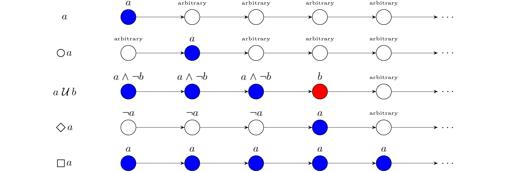
For the temporal operators, the semantics can be visualized as below:

From LTL to $\omega$-regular languages

Previous chapter: Linear-Time Temporal Logic (LTL)

This is a learning note of a course in CISPA, UdS. Taught by Bernd Finkbeiner

Introduction

In this section, we consider again our concurrent program $\small{\text{TURN}}$ introduced in section 1.1. As discussed before, a major property of interest is mutual exclusion,i.e., at any given point of time, at most one process is in the $\text{critical}$ region. We can express mutual exclusion, as well as other properties of turn, in LTL.

$\textbf{Example 1.1. }\small{\text{TURN}}:$
$$\text{local $t$: boolean where initially $t$ = $false$}\newline
P_0::\left[ \begin{array}{l}\text{loop forever do}\newline
\hspace{1cm}\left[ \begin{array}{l}
\ell_0: \text{await }\neg t; \newline
\ell_1: \text{critical;} \newline
\ell_2: t := true; \newline
\end{array} \right]\end{array} \right]
\mid\mid P_1::\left[ \begin{array}{l}
\text{loop forever do}\newline
\hspace{1cm}\left[ \begin{array}{l}
m_0: \text{await } t; \newline
m_1: \text{critical;} \newline
m_2: t := false; \newline
\end{array} \right]\end{array} \right]$$

Properties of the Concurrent Program $\small{\text{TURN}}$

Mutual exclusion : $\square\neg(\ell_1\wedge m_1)$

$\ell_{1}$ and $m_1$ cannot ($\neg$) be true at the same time ($\wedge$) at every point in time ($\square$)

The property can equivalently be formulated as $\neg(\textit{true}\ \mathcal{U}\ (\ell_1\wedge m_1))$, which means that the system remains true, until the a violation of mutual exclusion, i.e., $\ell_1\wedge m_1$, occurs

Finite waiting : $\square((\ell_0\rightarrow\Diamond\ell_1)\wedge(m_0\rightarrow\Diamond m_1))$

Previous chapter: Complement Büchi Automaton with Odd Ranking

This is a learning note of a course in CISPA, UdS. Taught by Bernd Finkbeiner

Introduction

In the following sections, we introduce several logics for the specification of sets of infinite sequences: LTL, QPTL, and S1S, which can be used to describe $\omega$-regular languages: we can translate a given formula into an automaton that recongnizes the models of the formula.

As a result, we can use the automata-theoretic machinery to answer logical questions like satisfiability or validity. We can also use the logics as a much more convenient starting point, compared to a direct specification using automata, for verification and synthesis.

Linear-Time Temporal Logic (LTL)

Linear-time temporal logic (LTL) is a popular logic for the specification of reactive systems. For a given set of atomic propositions$(AP)$, the formulas of LTL define sets of infinite words over the alphabet $2^{AP}$.

• Atomic Propositions:
  the interface of a system or a component, such as (a boolean representation of) input and output variables
• Words defined by the Formula:
  the executions of the system that are considered correct (see example in section 1.1).

Syntax of LTL

φ has to be true until and including the point where ψ first becomes true; if ψ never becomes true, φ must remain true forever.

Previous chapter: Ranking of DAG

This is a learning note of a course in CISPA, UdS. Taught by Bernd Finkbeiner

Introduction

In section 4.2, we have shown the complementation construction for deterministic Büchi Automata.

Now, by using DAG we can construct complement automaton of any Büchi Automata, with the help of the definition of odd ranking and the new function Level Ranking.

Level Ranking

$\textbf{Definition 5.3. }\text{(Level Ranking). Consider a Büchi Automaton }\mathcal{A}=(\Sigma,Q,I,T,\small\text{BÜCHI}\normalsize(F)).\newline\text{A level ranking }\ell\text{ is a pair }(S,g)\text{ such that:}$
$\begin{array}{l}
\hspace{1cm} \cdot \ S\subseteq Q,\newline
\hspace{1cm} \cdot \ g:S\rightarrow\lbrace 0,\dots,2|Q|\rbrace\text{ with }g(q)\text{ necessarily even if }q\in F.\end{array}\newline \ \newline\text{We also denote: }$
$\begin{array}{lll}
\hspace{1cm} \cdot \ \textsf{Lvlrks}&=&\text{the (finite) set of level ranks, and }\newline
\hspace{1cm} \cdot \ \textsf{Initrks}&=&\text{the set of level ranks s.t. }S=I\end{array}\newline \ \newline
\hspace{1cm}\text{We say that a level ranking }\ell’\text{, given by }(S’,g’)\text{ cover }\ell\text{, given by }(S,g)\text{ for }\sigma\in\Sigma,\newline\text{if }S’=\lbrace q’\mid(q,\sigma,q’)\in T\rbrace\text{ and for all }q\in S,q’\in S’\text{ with }(q,\sigma,q’)\in T\text{, it holds that } g’(q’)\leq g(q).$

Here, the level ranking refers to a pair that contains set of states that share the same ranking.

$\ell’$ covers $\ell$ ?

The last part of the definition states that one level ranking is covering the other if the following satisfied:

Previous chapter: Infinite Directed Acyclic Graph (DAG)

This is a learning note of a course in CISPA, UdS. Taught by Bernd Finkbeiner

Ranking

last section, we have introduced the DAG and the pruning method to reason about the run of the word on a non-deterministic Büchi automaton. We know that pruning can be use to prove the non-acceptance of the word by automaton is we obtains an empty graph eventually.

In this section, we will introduce ranking, which can formalize our pruning construction.

$\textbf{Definition 5.2. }\text{(Ranking). A }\textit{ranking}\text{ on a run DAG } G=(V,E)\text{ is a function }f:V\rightarrow\newline\lbrace 0,\dots,2|Q|\rbrace\text{ such that:}$
$\begin{array}{l}\hspace{1cm} 1. \ \text{ If }q\in F\text{, then }f((q,i))\text{ is even for all }i.\newline\hspace{1cm} 2. \ \text{ If }(v,v’)\in E\text{, we have that }f(v’)\leq f(v).\end{array}\newline$
$\text{A ranking } f\text{ is }\textit{odd}\text{ if, for each even }j\text{, there is no infinite path in }G\text{ that consists only }\newline\text{of verticies }v\text{ such that }f(v)=j.$

By the above definition, we can see:

1. All verticies that contains state q (the accepting state) are marked as even rank.
2. Verticies will never have lower rank than their successors.

Most importantly, it introduced a new concept: Odd Ranking. Meaning that the run of the DAG is rejected.

Previous chapter: Complementation of deterministic Büchi Automata

This is a learning note of a course in CISPA, UdS. Taught by Bernd Finkbeiner

Reasoning about all runs of an automaton

Since complementation inevitably introduce nondeterminism, we need to check whether all runs of the automaton on the word are rejecting to determine whether a word is in the complement of the language recognized by this Büchi automaton.

Example

Consider the following nondeterministic Büchi automaton $\mathcal{A}$. Its language consists of all infinite words over $\lbrace a,b\rbrace$ with infinitely many bs, i.e., $(a^*b)^\omega$:

$\textbf{Definition 5.1. }\text{Let }\mathcal{A}=(\Sigma,Q,I,T,\small\text{BÜCHI} \normalsize(F))\text{ be a Büchi automaton. The run DAG of }\mathcal{A}\newline\text{on a word }\alpha\in\Sigma^\omega\text{ is the directed acylic graph }G=(V,E)\text{, where}$
$\begin{array}{lll}
\hspace{1cm} \cdot \ V&=&\cup_{i\geq0}(Q_i\times\lbrace i\rbrace)\text{ with }Q_0=I\text{ and}\newline
\hspace{1.1cm} \ Q_{i+1}&=&\lbrace q’\mid(q,\alpha(i),q’)\in T\text{ for some }q\in Q\rbrace\newline
\hspace{1cm} \cdot \ E&=&\lbrace((q,i),(q’,i+1))\mid i\geq 0,(q,\alpha(i),q’)\in T\rbrace.\end{array}$
$\text{For a natural number }i\text{, we refer to the set }Q_i\text{ as the }\textit{level }i\text{ of the DAG.}$

Using infinite directed acyclic graph (DAG) to represent the set of all runs on a particular word, e.g., $ababa^\omega$.

Previous chapter: Deterministic vs. Nondeterministic Büchi Automata

This is a learning note of a course in CISPA, UdS. Taught by Bernd Finkbeiner

Introduction

For regular languages, Complementation is very simple: one translates a given complete deterministic automaton $\mathcal{A}$ that recognizes some language $L\subseteq\Sigma^*$ into an automaton $\mathcal{A’}$ that recognizes the complement $\Sigma^*\setminus L$ by complementing the set of final states, i.e., $F’=Q\setminus F$.

For deterministic Büchi automata, the construction is tricky, because it introduces nondeterminism

$\textbf{Construction 4.1. }\text{Let }\mathcal{A}=(\Sigma,Q,I,T,\small\text{BÜCHI} \normalsize(F))\text{ be a complete deterministic Büchi}\newline\text{automaton, where we assume w.l.o.g. that } Q\neq\varnothing. \text{ We construct a Büchi automaton}\newline\mathcal{A’}=(\Sigma,Q’,I’,T’,\small\text{BÜCHI} \normalsize (F’))\text{ with }\mathcal{L}(\mathcal{A’})=\Sigma^\omega\setminus\mathcal{L}(\mathcal{A})\text{ as follows:}$
$\begin{array}{lrll}
\hspace{1cm} \cdot &Q’&=&(Q\times\lbrace 0\rbrace)\cup((Q\setminus F)\times\lbrace 1\rbrace)\newline
\hspace{1cm} \cdot &I’&=&I\times\lbrace 0\rbrace\newline
\hspace{1cm} \cdot &T’&=&\lbrace ((q,0),\sigma,(q’,i))\mid(q,\sigma,q’)\in T,i\in\lbrace 0,1\rbrace,(q’,i)\in Q’\rbrace \cup \newline
\hspace{1cm} \ &&&\lbrace ((q,1),\sigma,(q’,1))\mid(q,\sigma,q’)\in T,q’,q’\in Q\setminus F\rbrace\newline
\hspace{1cm} \cdot &F’&=&(Q\setminus F)\times\lbrace 1\rbrace
\end{array}$

	Explaination
$Q’$	Uses two copies of the given automaton $\mathcal{A}$, mark them seperately using $\lbrace 0\rbrace$ and $\lbrace 1\rbrace$, notice that all accpeting states from $\lbrace 1\rbrace$ are eliminated
$I’$	The complemented automaton starts from initial states from $\lbrace 0\rbrace$.
$T’$	The switch from $\lbrace 0\rbrace$ and $\lbrace 1\rbrace$ happens nondeterministically. And once you enter the second copy $\lbrace 1\rbrace$, it stays forever.
$F’$	The automaton $\mathcal{A’}$ accepts if the run ends up in the second copy, which means that, on the unique run of $\mathcal{A}$ on the input word, the accepting states of $\mathcal{A}$ are only visited finitely often.

Note that the resulting automaton is nondeterministic. This is, in general, unavoidable.

This is because there are languages, such as $L=(b^*a)^\omega$ where the language itself is recognizable by a deterministic Buchi automaton, while its complement $\Sigma^\omega\setminus L$ can only be recognized by a nondeterministic Büchi automaton.

$\textbf{Theorem 4.3. }\textit{For every deterministic Büchi automaton }\mathcal{A}\textit{, there exists a Büchi automaton }\mathcal{A’}\newline\textit{ such that }\mathcal{L}(\mathcal{A’})=\Sigma^\omega \setminus\mathcal{L}(\mathcal{A}).$

Previous chapter: Büchi’s Characterization Theorem

This is a learning note of a course in CISPA, UdS. Taught by Bernd Finkbeiner

Introduction

In the theory of automata over finite words, we have Rabin-Scott powerset construction, which converts a nondeterministic automaton over finite words into a deterministic automaton that recognizes the same language. This shows that nondeterminism does not make automata over finite words more expressive (but makes it more concise as the construction produces an exponential number of states).

The situation is different for Büchi automata: even though the language $L = (a+b)^*b^\omega$ is clearly Büchi-recognizable, there is, as the following theorem shows, no deterministic Büchi automaton that recognizes L.

Deterministic vs. nondeterministic Büchi automata

$\textbf{Theorem 4.1. }\textit{Language $L=(a+b)^*b^\omega$ is not recognizable by deterministic Büchi Automata}$

Starting a base case $b^\omega$, we add $(a+b)$ as the prefix one by one. Can we express the kleene star?
That is, is the automaton only accept finitely many $(a+b)$?

Proof

Assume, by way of contradiction, that $L$ is recognizable by the deterministic Büchi automaton $\mathcal{A}=(\Sigma,Q,I,T,\small\text{BÜCHI}\normalsize(F))$. Since $\alpha_0=b^\omega$ is in $L$, there is an unique run