Previous chapter: Infinite Games (Basic Definitions)

This is a learning note of a course in CISPA, UdS. Taught by Bernd Finkbeiner

Reachability Condition

We will now analyze infinite games for various types of winning conditions. We start with the simple reachability condition.

The reachability condition is given as a set $R$ of positions called the reachability set. The reachability condition is satisfied if the play reaches some position in $R$. Formally, for an infinite word $\alpha$ over $\Sigma$, we use $\text{Occ}(\alpha) := \lbrace\sigma\in\Sigma\mid\exists n\in\mathbb{N}.\ \alpha(n)=\sigma\rbrace$ to denote the set of all letters occurring in $\alpha$.

$\textbf{Definition 11.11. } \text{The }\textit{reachability condition }\small\text{REACH} \normalsize(R)\text{ on a set of positions }R\subseteq V\text{ is the set}$

$$ \small\text{REACH} \normalsize(R) = \lbrace\rho\in V^\omega\mid\text{Occ}(\rho)\cap R\neq\varnothing\rbrace$$
$$\text{A game }\mathcal{G}=(\mathcal{A},\text{Win})\text{ with Win}=\small\text{REACH} \normalsize(R)\text{ is called a }\textit{reachability game}\text{ with reachability set }R $$

Example

$$
\text{Position of Player 0: Circles;}\ \ \text{Positions of Player 1: rectangles.}$$

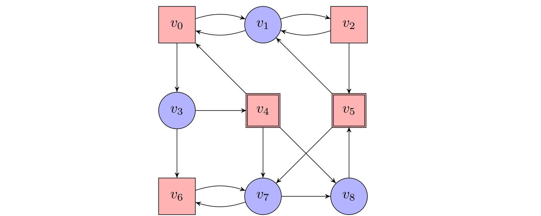
$$\mathcal{G}=(\mathcal{A},\small\text{REACH} \normalsize(R)),\ R=\lbrace v_4,v_5\rbrace
$$

Previous chapter: From semi-deterministic Büchi to deterministic Muller

This is a learning note of a course in CISPA, UdS. Taught by Bernd Finkbeiner

Introduction

We now introduce infinite two-player games on finite graphs. Infinite games are useful to solve the synthesis problem, where we are interested in finding a strategy that guarantees that a given specification is satisfied (cf. Section 1.2). As we will see, games also play a fundamental role in automata theory, in particular for automata over infinite trees.

Basic Definitions

The game is played on a graph, called the arena. The vertices of the graph are called positions and are partitioned into the positions of Player 0 and the positions of Player 1.

• A play of the game starts in some initial position
• In any positions, the player who owns the position chooses the edge on which the play is continued.
• Player 0 wins if the play is an element of the winning condition.

The winner is determined by a winning condition, which, like the acceptance condition of an automaton on infinite words is a subset of the infinite words over the positions.

$\textbf{Definition 11.1. } \text{A }\textit{game arena}\text{ is a tuple }\mathcal{A} = (V,V_0,V_1,E)\text{, where}$

$\begin{array}{l}
\hspace{0.5cm} \cdot \ V_0\text{ and }V_1=V\setminus V_0\text{ are disjoint sets of positions,}\newline
\hspace{1cm} \text{called the positions of Player 0 and Player 1.}\newline
\hspace{0.5cm} \cdot \ E\subseteq V\times V\text{ is a set of edges such that every position }v\in V\newline
\hspace{1cm} \text{has at least one outgoing edge }(v,v’)\in E.\newline
\end{array}$

$\textbf{Definition 11.2. } \text{A }\textit{play}\text{ is an infinite sequence } \rho\in V^\omega\text{ such that}$
$$\forall n\in\mathbb{N}.(\rho(n),\rho(n+1))\in E$$

Previous chapter: Semi-Deterministic Büchi Automata

This is a learning note of a course in CISPA, UdS. Taught by Bernd Finkbeiner

Introduction

From the semi-deterministic Büchi automaton we now build a deterministic Muller automaton. The idea of the construction is to continuously simulate, in the deterministic automaton, the nondeterministic part of the semi-deterministic automaton and to ”attempt” a transition into the deterministic part whenever possible.

In the state of the deterministic automaton we maintain an “array” of states that correspond to these attempts. Along each run of the automaton, there may of course be infinitely many such attempts; we only need a finite array, however, because we do not need to keep track of two different attempts to enter the deterministic part, if they both reach the same state (in this case, we simply track the attempt that entered the deterministic part earlier).

We use an array of size $2m$, where m is the number of states of the deterministic part. The factor two allows us to leave a position of the array empty (“␣”) if an attempt is not continued. This is necessary to distinguish a situation where a previously started attempt failed and, at the same time, a new attempt enters the deterministic part, from the situation where the same attempt ran continuously. The deterministic automaton accepts if there is at least one attempt that runs forever after some point and reaches an accepting state infinitely often.

---

Next chapter: Infinite Games (Basic Definitions)

Further Reading:

Previous chapter: Closure Properties of Muller automata Under Boolean Operations

This is a learning note of a course in CISPA, UdS. Taught by Bernd Finkbeiner

Introduction

To prove McNaughton’s theorem, in this subsection, we will introdue the semi-deterministic Büchi automata.

1. translate nondeterministic Büchi automata into semi-deterministic Büchi automata.
2. translate from semi-deterministic Büchi automata to deterministic Muller automata.

Semi-deterministic Büchi Automata

A semi-deterministic automaton is a (possibly nondeterministic) automaton where all accepting runs ultimately end up in a subset of the states from which all transitions are deterministic.

$\textbf{Definition 10.2. } \text{A Büchi automata }\mathcal{A} = (\Sigma,Q,I,T,\small\text{BÜCHI} \normalsize(F))\text{ is }\textit{semi-deterministic}\text{ if}$ $ Q = N \uplus D\text{ is a partition of }Q\text{ such that }F\subseteq D, pr_2(T\cap(D\times\Sigma\times Q))\subseteq D\text{, and }$ $(\Sigma,D,\lbrace d\rbrace,T\cap(D\times\Sigma\times D),\small\text{BÜCHI}\normalsize(F)) \text{ is deterministic for every }d\in D.$

Explaination

$Q = N \uplus D:$ a disjoint union symbol $\uplus$ indicates that $N$ and $D$ are two seperated subset.

Previous Exercise:

This is a learning note of a course in CISPA, UdS. Taught by Bernd Finkbeiner

This is an example exercise to express LTL formula into Alternating Büchi Automata. For further definitions, you may check Section 7.2.

Question

Use the construction from the lecture to construct an alternating Büchi automaton $\mathcal{A}$ such that $$\mathcal{L(A)=L}((\Diamond p)\ \mathcal{U}\ (\square q))$$

Solution

we build the following alternating Büchi automaton $\mathcal{A} = (2^{p,q},Q,\varphi,\delta,\small\text{BÜCHI} \normalsize(F))$ which recognizes the models of $\varphi=(\Diamond p)\ \mathcal{U}\ (\square q)$. First we consider the transition function $\delta$ for an arbitrary symbol $a\in2^{p,q}:$

$\begin{array}{lll}
\hspace{1cm}\bullet &&\delta(\square q,a)\newline
&=&\delta(\neg(\textit{true}\ \mathcal{U}\ \neg q) ,a)\newline
&=&\overline{\delta(\textit{true}\ \mathcal{U}\ \neg q ,a)}\newline
&=&\overline{\delta(\neg q,a)\vee(\delta(\textit{true},a)\wedge(\textit{true}\ \mathcal{U}\ \neg q))}\newline
&=&\overline{\delta(\neg q,a)}\wedge\overline{(\delta(\textit{true},a)\wedge (\textit{true}\ \mathcal{U}\ \neg q))}&(\textit{true}\wedge \psi=\psi)\newline
&=&\overline{\delta(\neg q,a)}\wedge\overline{(\textit{true}\ \mathcal{U}\ \neg q)}&(\text{Using line 1})\newline
&=&\overline{\delta(\neg q,a)}\wedge\square q\newline
&=&\left\lbrace \begin{array}{lll}
\square q&\text{if }q\in a\newline
\textit{false}&\text{if }q\notin a\newline
\end{array}\right.
\end{array}
\ \newline \ \newline
\begin{array}{lll}
\hspace{1cm}\bullet &&\delta(\Diamond p,a)\newline
&=&\delta(\textit{true}\ \mathcal{U}\ p ,a)\newline
&=&\delta(p,a)\vee(\delta(\textit{true},a)\wedge\Diamond p)&(\textit{true}\wedge \psi=\psi)\newline
&=&\delta(p,a)\vee\Diamond p\newline
&=&\left\lbrace \begin{array}{lll}
\Diamond p&\text{if }p\notin a\newline
\textit{true}&\text{if }p\in a\newline
\end{array}\right.
\end{array}
$

By Substitution above result into $\delta((\Diamond p)\ \mathcal{U}\ (\square q),a)=\delta(\square q,a)\vee(\delta(\Diamond p,a)\wedge(\Diamond p)\ \mathcal{U}\ (\square q))$, we have:

$$\delta((\Diamond p)\ \mathcal{U}\ (\square q),a)=\left\lbrace
\begin{array}{lll}
\Diamond p\wedge((\Diamond p)\ \mathcal{U}\ (\square q))&\text{if }a =\varnothing &(\vee\ \textit{false}\text{ is omitted.})\newline
(\Diamond p)\ \mathcal{U}\ (\square q)&\text{if }a =\lbrace p\rbrace&(\wedge\ \textit{true}\text{ is omitted.})\newline
\square q\vee(\Diamond p\wedge((\Diamond p)\ \mathcal{U}\ (\square q)))&\text{if }a =\lbrace q\rbrace\newline
\square q\vee((\Diamond p)\ \mathcal{U}\ (\square q))&\text{if }a =\lbrace p,q\rbrace&(\wedge\ \textit{true}\text{ is omitted.})\newline
\end{array}\right.$$

Previous chapter: From Büchi automata to Muller automata

This is a learning note of a course in CISPA, UdS. Taught by Bernd Finkbeiner

Introduction

We now show that deterministic Muller automata are closed, like nondeterministic Büchi automata, under the Boolean operations (complementation, union, and intersection).

First we introduce the construction of these automaton with operations, then we will prove they are close by the runs under those constructions.

Automata construction of Complementation

$\textbf{Construction 10.3. } \text{Let }\mathcal{A} = (\Sigma,Q,I,T,\small\text{MULLER} \normalsize (\mathcal{F}))\text{ be a complete and deterministic Muller}$ $\text{automaton, where we assume w.l.o.g that }Q\neq\varnothing.\text{ We construct the deterministic Muller}$ $\text{automaton }\mathcal{A}^C = (\Sigma,Q,I,T,\small\text{MULLER} \normalsize(2^Q\setminus\mathcal{F}))\text{ with }\mathcal{L(A^C)}=\Sigma\setminus\mathcal{L(A)}.$

Automata construction of Intersection

We use the function $pr_n$ for $n\in\mathbb{N}$ to project to the (n+1)th component of a arbitrary length tuple, for example:

• $pr_0(x, y)=x$
• $pr_1(x, y)=y$
• $pr_2(x, y),pr_3(x, y),\dots pr_n(x, y) =\text{Undefined}$

Previous chapter: The Muller Acceptance Condition

This is a learning note of a course in CISPA, UdS. Taught by Bernd Finkbeiner

In this section, we want to prove that Muller automata is equivalent to Büchi Automata.

Translate Büchi Automata into Muller Automata

$\textbf{Construction 10.1. } \text{For a (deterministic) Büchi Automaton }\mathcal{A} = (\Sigma,Q,I,T,\small\text{BÜCHI}\normalsize (F))$ $\text{ we define the (deterministic) Muller automaton } \mathcal{A’} = (\Sigma,Q,I,T,\small\text{MULLER} \normalsize (\mathcal{F}))\text{ using}$

$$\mathcal{F}=\lbrace S\subseteq Q\mid S\cap F\neq\varnothing\rbrace$$

Since the construction does not modify the transitions, the Muller automaton is again deterministic if the Büchi automaton is deterministic. It is straightforward to see that the automata recognize the same language.

$\textbf{Theorem 10.1. } \textit{For every (deterministic) Büchi automaton }\mathcal{A}\textit{, there is a (deterministic)}$ $\textit{Muller automaton }\mathcal{A’}\textit{ such that }\mathcal{L(A)}=\mathcal{L(A’)}.$

Proof

The automaton $\mathcal{A’}$ of Construction 10.1 complies with our requirements, according to previous section:

$$\small\text{BÜCHI}\normalsize (F)=\lbrace\alpha\in Q^\omega\mid\text{Inf}(\alpha)\cap F\neq\varnothing\rbrace=\lbrace\alpha\in Q^\omega\mid\text{Inf}(\alpha)\in\mathcal{F}\rbrace=\small\text{MULLER}\normalsize(\mathcal{F})$$

Previous chapter: The Emerson-Lei algorithm

This is a learning note of a course in CISPA, UdS. Taught by Bernd Finkbeiner

Introdcution

We already established that while the languages that can be recognized with nondeterministic Büchi automata are exactly the $\omega$-regular languages, the languages that can be recognized with deterministic Büchi automata are a strictly smaller set.

We now repair this deficiency with a more expressive acceptance condition, the Muller condition. McNaughton’s theorem states that the set of languages recognizable by deterministic Muller automata are again exactly the $\omega$-regular languages.

We will see later that it is very useful to have a deterministic automaton for a given $\omega$-language, for example in synthesis, where we construct the game between the system and the environment from a deterministic automaton that recognizes the winning plays for the system player.

Since the complementation of deterministic Muller automata is a very simple operation, McNaughton’s theorem also provides an alternative proof for the result of Section 5 that the $\omega$-regular languages are closed under complementation.

Muller Acceptance Condition

$\textbf{Definition 10.1. } \text{The }\textit{Muller Acceptance Condition }\small\text{MULLER} \normalsize(\mathcal{F})\text{ on a set of sets of states }$ $\mathcal{F}\subseteq 2^Q\text{ is the set}$

$$\small\text{MULLER}\normalsize(\mathcal{F})=\lbrace\alpha\in Q^\omega\mid\text{Inf}(\alpha)\in\mathcal{F}\rbrace$$

$\text{An automaton }\mathcal{A} = (\Sigma,Q,I,T,Acc) \text{ with }Acc = \small\text{MULLER} \normalsize(\mathcal{F})\text{ is called a }\textit{Muller Automaton.}$ $\text{The set }\mathcal{F}\text{ is called the set of }\textit{accepting subsets }(\text{or the }\textit{table})\text{ of }\mathcal{A}.$

Let’s do a small recap from section 2.3:

Previous chapter: Nested depth-first search

This is a learning note of a course in CISPA, UdS. Taught by Bernd Finkbeiner

Introduction

As an alternative algorithm for checking language emptiness of Büchi automata we now discuss a classic algorithm due to Emerson and Lei. Unlike the depth-first search of the previous subsection, the Emerson-Lei algorithm is based on a breadth-first search implemented as a fixpoint construction over sets of states.

A disadvantage of this algorithm is that its running time is quadratic. Nevertheless, algorithms of this type play a major role in symbolic model checking, because the sets of states can often be represented efficiently
using data structures like binary decision diagrams.

Live states

A state $q$ of a Büchi automaton is live if some infinite path starting in $q$ visits accepting states infinitely often. This definition is the opposite of safe states, where it never visits accepting states. The idea of the algorithm is to identify the set of live states. The language of a Büchi automaton is non-empty iff it has a live initial state.

The Emerson-Lei algorithm is based on the following inductive definition:

$\textbf{Definition 9.1. } \text{For a Büchi automaton and a number }n\in\mathbb{N}\text{, the set of }\textit{n-live states}\text{ is}$ $\text{defined as follows:}$

$\begin{array}{l}
\hspace{1cm}\cdot\ \text{every state is 0-live}\newline
\hspace{1cm}\cdot\ \text{a state q is (n + 1)-live if some path containing at least one transition leads from }q\newline\hspace{1.3cm}\text{to an accepting n-live state}\newline
\end{array}$

Fixpoint

Previous chapter: Automata-based LTL Model Checking with Sequential Circuits

This is a learning note of a course in CISPA, UdS. Taught by Bernd Finkbeiner

Introduction

We now develop an algorithm for checking whether the language of a given Büchi automaton is empty. A natural idea is to use depth-first search (DFS) twice.

The language is non-empty $\Leftrightarrow$ it is accepted by some words:

1. there exists an accepting state $q$,
2. $q$ is reachable from some initial state (discovered by 1st DFS), and
3. $q$ can again be reached from $q$ (discovered by 2nd DFS),

Example (Simple DFS)

Consider the following Büchi automaton (edge labels do not matter and are omitted).

Step 1: discovers $q_0$, $q_1$, and $q_3$.
Step 2: searches from $q_0$ and $q_3$: not successful; searches from $q_1$: discovers the path back to $q_1$ via $q_2$.